Enhanced Sampling Simulations
with Ensembler
In this notebook, we give examples for enhanced sampling simulations with Ensembler. We show how to execute, visualize, and analyze those simulations for both 1D and 2D systems.
The enhanced sampling technologies are briefly explained in order to directly use this notebook for teaching purpose.
Maintainers: [@SchroederB](https://https://github.com/SchroederB), [@linkerst](https://https://github.com/linkerst), [@dfhahn](https://https://github.com/dfhahn)
Loading Ensembler and necessary external packages
[1]:
import os, sys
my_path = os.getcwd()+"/.."
sys.path.append(my_path)
import matplotlib
matplotlib.use('TkAgg')
import numpy as np
%matplotlib inline
from matplotlib import pyplot as plt
from ensembler.potentials.OneD import fourWellPotential, harmonicOscillatorPotential, addedPotentials, metadynamicsPotential
from ensembler.potentials.TwoD import harmonicOscillatorPotential as harmonicOscillator2D, wavePotential as wavePotential2D, gaussPotential
from ensembler.potentials.TwoD import addedPotentials as addedPotentials2D, metadynamicsPotential as metadynamicsPotential2D
from ensembler.samplers.stochastic import langevinIntegrator, langevinVelocityIntegrator
from ensembler.system import system
from ensembler.ensemble import replica_exchange
##Visualisation
from ensembler.visualisation.plotSimulations import simulation_analysis_plot
Enhanced Sampling Simulations in 1D
Unbiased System
We start our walkthrough with an unbiased reference simulation of a four-well-potential and give a small introduction in how to set up a simulation with Ensembler. The four-well-potential is defined by the x-positions (\(a\)-\(d\)) and the y-position \(ah\) - \(dh\) of the four wells. If wished, the potential can be scaled in the y-direction using \(V_{max}\). Note, that the energy is given in units of \(k_BT\).
[2]:
# Simulation Setup
pot = fourWellPotential(Vmax=4, a=1.5, b=4.0, c=7.0, d=9.0, ah=2., bh=0., ch=0.5, dh=1.)
Here, we choose the stochastic Langevin integrator for the numeric integration of our system. The user has to set the step size \(dt\) and the friction coefficient \(gamma\). Note, that this integrator already contains a thermostat. The temperature of the simulation will be set during the system setup (see below).
[3]:
# Simple Langevin integration simulation
integrator = langevinIntegrator(dt=0.1, gamma=15)
The system class wraps the integrator and the potential. Additionally, the initial position of the particle \(position\) as well as the temperature parameter \(temperature\) are set.
[4]:
# Put Potential and Integrator together to generate the simulation system
system1 = system(potential=pot, sampler=integrator, start_position=4.2, temperature=1)
To start the simulation we define the number of steps and run sys.simulate(). The progress of the simulation is displayed by a progress bar.
[5]:
#simulate
sim_steps = 2000
cur_state = system1.simulate(sim_steps, withdraw_traj=True, init_system=False)
print("Trajectory length: ",len(system1.trajectory))
print()
print("last_state: ", cur_state)
print(len(system1.trajectory))
Simulation: Simulation: 0%| | 0/2000 [00:00<?, ?it/s]
initializing Langevin old Positions
Simulation: Simulation: 100%|██████████| 2000/2000 [00:00<00:00, 4493.46it/s]
Trajectory length: 2001
last_state: State(position=3.9425114367580365, temperature=1, total_system_energy=0.011614955016301127, total_potential_energy=0.011614955016301127, total_kinetic_energy=nan, dhdpos=0.36274802794719235, velocity=None)
2001
After running the simulation, the simulation data can be displayed as a table using sys.trajectory. Note, that we used a position Langevin integrator that did not calculate the velocities explicitly. Therefore, the kinetic energy and velocity are not defined. If you want to calculate the velocities during the simulation use the langevinVelocityIntegrator instead.
[6]:
system1.trajectory.head()
[6]:
| position | temperature | total_system_energy | total_potential_energy | total_kinetic_energy | dhdpos | velocity | |
|---|---|---|---|---|---|---|---|
| 0 | 4.200000 | 1 | 0.158629 | 0.158622 | 0.000008 | 1.595959 | -0.003895 |
| 1 | 4.165484 | 1 | 0.108275 | 0.108275 | NaN | -1.595959 | NaN |
| 2 | 4.125017 | 1 | 0.061324 | 0.061324 | NaN | -1.321306 | NaN |
| 3 | 4.230917 | 1 | 0.211764 | 0.211764 | NaN | -0.999128 | NaN |
| 4 | 4.118459 | 1 | 0.054943 | 0.054943 | NaN | -1.841802 | NaN |
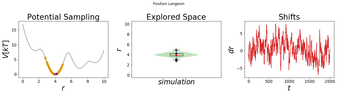
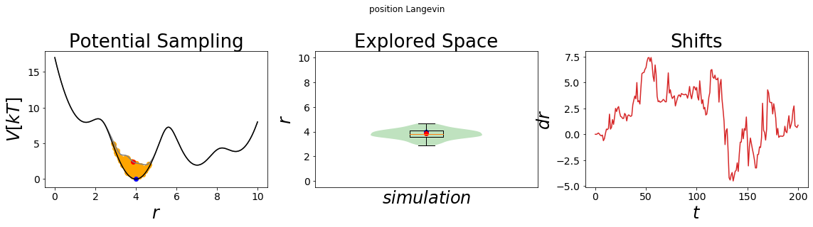
The simulation results can be visualized using the build-in visualizing tool. The left panel displays the energy surface as well as all visited states. The start and end-state are colored in blue and red, respectively. The middle panel shows the probability density distribution of the simulation as well as a boxplot of the distribution. This plot can be used to check if the system was simulated successfully. The rightmost panel shows the development of the force over time.
Note that without enhanced sampling only the minimum around x=4 is sampled. It would require a very long simulation time to overcome the energetic barrier and hence a lot of computing time. Enhanced sampling methods were developed to speed up those slow processes. We will explore some of the most commonly used enhanced sampling methods in the subsequent notebook.
[7]:
#plot
simulation_analysis_plot(system1, title="Position Langevin", limits_coordinate_space=list(range(0,10)))
[7]:
(<Figure size 1152x288 with 3 Axes>, None)
Enhanced sampling
Enhanced sampling methods can be divided into time-independent and time-dependent methods. Time-independent biases stay the same throughout the whole simulation whereas for time-dependent enhanced sampling the bias is updated during the simulation time.
Time-independent bias
Umbrella sampling
Umbrella sampling is a time-independent enhanced sampling method. In this method energy barriers are overcome by adding a bias potential. Note that umbrella sampling requires the choice of a reaction coordinate along which the bias is added. The choice of a suitable reaction coordinate is non-trivial for high dimensional systems. For our low dimensional 1D we can simply chose the x-axis.
One of the most frequent umbrella sampling method uses hormonic potentials to restrain the sampling to a certain region of the potential. This is especially useful for sampling transition regions.
We start as in the unbiased case by defining the potential. However, we have to define two potentials; the original potential and the bias potential. The original potential is the same potential as defined above, the bias potential is a hormonic oscillator centered at \(x_{shift}\) and force constant \(k\). In this case we want to sample the transition region around \(x\) = 5.5. Therefore, we set the \(x_{shift}\) parameter to 5.5. The force constant \(k\) defines how much we constrain the system. The higher the energy barrier, the more constrain is needed.
To sample the full potential energy landscape, we can set up multiple simulations with different \(x_{shift}\) parameters. For subsequent analysis of umbrella sampling simulations (e.g. using the weighted histogram analysis method WHAM) it is important that the sampling space of the different simulations overlap. The higher the force constant \(k\), the more simulations are needed achieve the overlap.
[8]:
#Simulation Setup
origpot = fourWellPotential(Vmax=4, a=1.5, b=4.0, c=7.0, d=9.0, ah=2., bh=0., ch=0.5, dh=1.)
biaspot = harmonicOscillatorPotential(k=10, x_shift=5.5)
The addedPotentials function of the biasOneD class wraps any two 1D potentials together. Therefore, it is straightforward to generate the enhanced sampling system from the original and biased potential.
[9]:
#Add the bias and the original system
totpot = addedPotentials(origpot, biaspot)
All subsequent steps are identical to the unbiased system. Note, that the starting position of the simulation has to match to the \(x_{shift}\) parameter (i.e. should be reasonable close to \(x_{shift}\)) in order to avoid starting the simulation at very high energy states.
[10]:
integrator = langevinIntegrator(dt=0.1, gamma=15)
system2 = system(potential=totpot, sampler=integrator, start_position=4.2, temperature=1)
#simulate
sim_steps = 2000
cur_state = system2.simulate(sim_steps, withdraw_traj=True, init_system=False)
print("Trajectory length: ",len(system2.trajectory))
print()
print("last_state: ", cur_state)
print(len(system2.trajectory))
system2.trajectory.head()
Simulation: Simulation: 0%| | 0/2000 [00:00<?, ?it/s]
initializing Langevin old Positions
Simulation: Simulation: 100%|██████████| 2000/2000 [00:01<00:00, 1634.03it/s]
Trajectory length: 2001
last_state: State(position=4.805903751721836, temperature=1, total_system_energy=4.969236534763127, total_potential_energy=4.969236534763127, total_kinetic_energy=nan, dhdpos=0.7439640744837144, velocity=None)
2001
[10]:
| position | temperature | total_system_energy | total_potential_energy | total_kinetic_energy | dhdpos | velocity | |
|---|---|---|---|---|---|---|---|
| 0 | 4.200000 | 1 | 8.609497 | 8.608622 | 0.000875 | -11.404041 | -0.04184 |
| 1 | 4.285465 | 1 | 7.699532 | 7.699532 | NaN | 11.404041 | NaN |
| 2 | 4.495405 | 1 | 6.021825 | 6.021825 | NaN | 9.870341 | NaN |
| 3 | 4.505998 | 1 | 5.958023 | 5.958023 | NaN | 6.117316 | NaN |
| 4 | 4.614714 | 1 | 5.418150 | 5.418150 | NaN | 5.928966 | NaN |
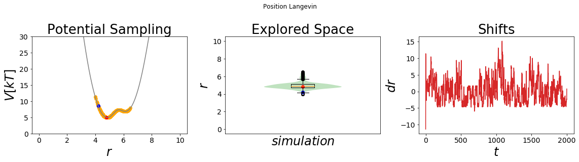
In order to visualize the resulting potential we again use the plotting function simulation_analysis_plot. The visualization shows that umbrella sampling samples the high energy transition region around x=5.5 very well. In contrast, the unbiased simulation (see above) was stuck at the minimum around x=4.
[11]:
#plot
simulation_analysis_plot(system2, title="Position Langevin", limits_coordinate_space=list(range(0,10)), oneD_limits_potential_system_energy=[0,30])
[11]:
(<Figure size 1152x288 with 3 Axes>, None)
Scaled potential
addedPotentials can add any potential classes with a given dimensionality. In the special case that the added potential is identical to the original potential but a prefactor, one can scale the potential. In the example below we chose a four well potential that we will scale down in order to cross the energy barriers more easily. The procedure to define the original and bias potential are the same as described above.
[12]:
sim_steps = 2000
#Simulation Setup
origpot=fourWellPotential(Vmax=4, a=1.5, b=4.0, c=7.0, d=9.0, ah=2., bh=0., ch=0.5, dh=1.)
# same potential but Vmax is different
biaspot = fourWellPotential(Vmax=-3.5, a=1.5, b=4.0, c=7.0, d=9.0, ah=2., bh=0., ch=0.5, dh=1.)
#Add the bias and the original system
totpot = addedPotentials(origpot, biaspot)
integrator = langevinIntegrator(dt=0.1, gamma=15)
system3=system(potential=totpot, sampler=integrator, start_position=4.2, temperature=1)
#simulate
cur_state = system3.simulate(sim_steps, withdraw_traj=True, init_system=False)
print("Trajectory length: ",len(system3.trajectory))
print()
print("last_state: ", cur_state)
print(len(system3.trajectory))
system3.trajectory.head()
Simulation: Simulation: 0%| | 0/2000 [00:00<?, ?it/s]
initializing Langevin old Positions
Simulation: Simulation: 100%|██████████| 2000/2000 [00:01<00:00, 1657.18it/s]
Trajectory length: 2001
last_state: State(position=6.201177145687366, temperature=1, total_system_energy=0.556710481208582, total_potential_energy=0.556710481208582, total_kinetic_energy=nan, dhdpos=0.6806167726988884, velocity=None)
2001
[12]:
| position | temperature | total_system_energy | total_potential_energy | total_kinetic_energy | dhdpos | velocity | |
|---|---|---|---|---|---|---|---|
| 0 | 4.200000 | 1 | 0.021572 | 0.019828 | 0.001744 | 0.199495 | -0.059064 |
| 1 | 3.993458 | 1 | -0.000150 | -0.000150 | NaN | -0.199495 | NaN |
| 2 | 4.085934 | 1 | 0.003545 | 0.003545 | NaN | 0.006084 | NaN |
| 3 | 3.935761 | 1 | 0.001858 | 0.001858 | NaN | -0.085983 | NaN |
| 4 | 3.871948 | 1 | 0.007934 | 0.007934 | NaN | 0.063492 | NaN |
[13]:
#plot
simulation_analysis_plot(system3, title="position Langevin", limits_coordinate_space=list(range(0,12)))
[13]:
(<Figure size 1152x288 with 3 Axes>, None)
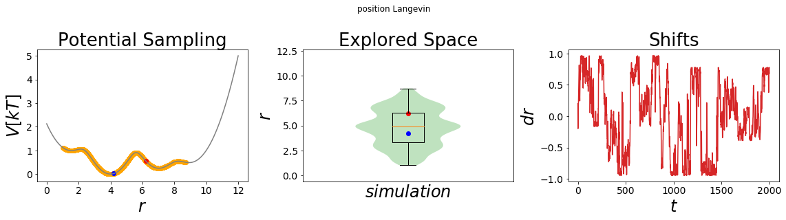
Through the visualization we get the confirmation that we scaled the original potential down to 12.5% of its original height (first panel, compare the y-axis). Accordingly, the system has now enough thermal energy to cross all energy barriers and all four minima can be sampled.
Temperature Replica Exchange / Parallel Tempering
Temperature replica exchange, also called parallel tempering, is an enhanced sampling method that runs multiple copies of the simulated system at different temperatures. After a specific number of simulation steps, the current coordinate is exchanged with a simulation at a different temperature. However, this exchange is only triggered if a certain condition, e.g. the Metropolis criterion, is fulfilled. This approach has the advantage that one can couple high temperature simulations, that cross energy barriers quickly, with lower temperature systems that sample the minima. Therefore, thermodynamic properties can be calculated with higher precision as more local minima can be explored.
In our example we will perform a temperature replica exchange simulation with two systems. The temperatures of these two systems are defined by the \(T\_values\) parameter. We first define how many simulation steps we run per replica and how often the system should try to exchange the coordinates (\(simulation\_steps\_total\_per\_approach\) and \(trials\)). We wrap our system with the replica exchange conditions using the \(replica\_exchange.temperatureReplicaExchange\) class. Other replica methods covered in the Ensembler package are Hamiltonian replica exchange and Replica Exchange Enveloping Distribution Sampling (REEDS). REEDS is explained in the Free energy example notebook.
For our example simulation we use a common metropolis monte carlo criterium for RE approaches exchanging the coordinates of replica i and replica j,
\(p_{ij} = min(1, e^{(H_{i}(r_j)+H_{j}(r_i))-(H_{i}(r_i)+H_{j}(r_j))})\)
Note that every second trial is not accepted, as the algorithm alternates the partner of the pairwise exchange. Therefore every second exchange is a border exchange, which is in this case of two replicas not exchanging at al.=l. Subsequently, the simulation is performed as in our previous examples. As the langevine sampler is not calculating any kinetic energy, every exchange is accepted with this criterium.
[14]:
##Ensemble Settings:
T_values = np.array([100, 0.01])
simulation_steps_total_per_approach = 2000
trials = 10
steps_between_trials = simulation_steps_total_per_approach//trials
print("DO trials: ", trials, "steps: ", steps_between_trials)
#Simulation Setup
origpot=fourWellPotential(Vmax=4, a=1.5, b=4.0, c=7.0, d=9.0, ah=2., bh=0., ch=0.5, dh=1.)
integrator = langevinIntegrator(dt=0.1, gamma=15)
system_replica = system(potential=origpot, sampler=integrator, start_position=4.2, temperature=1)
#define the replica exchange criteria
ensemble = replica_exchange.temperatureReplicaExchange(system=system_replica, temperature_range=T_values,
exchange_criterium=None, steps_between_trials=steps_between_trials)
#simulate
cur_state = ensemble.simulate(trials, reset_ensemble=True)
replica_trajs = ensemble.replica_trajectories
DO trials: 10 steps: 200
Running trials: 0%| | 0/10 [00:00<?, ?it/s]
initializing Langevin old Positions
initializing Langevin old Positions
Running trials: 100%|██████████| 10/10 [00:02<00:00, 3.50it/s]
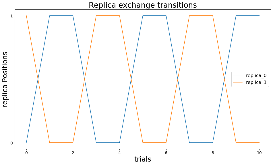
We first visualize the exchanges that occur during our simulations. In the figure below we observe that a single simulation with a fixed temperature (called replica) changes its coordinates multiple times. Indeed, the state is changed every second exchange trial. This is due to the \(exchange\_criterium=None\) setting.
[15]:
stats= ensemble.exchange_information
replicas = np.unique(ensemble.exchange_information.replicaID)
trials = np.unique(ensemble.exchange_information.nExchange)
import itertools as it
fig, ax = plt.subplots(ncols=1, figsize=[16,9])
replica_positions = {}
for replica in replicas:
replica_positions.update({replica: stats.loc[stats.replicaID==replica].replicaPositionI})
x = trials
y = replica_positions[replica]
ax.plot(x,y , label="replica_"+str(replica))
#plt.yticks(replicas+1, reversed(replicas+1))
ax.set_yticks(ticks=replicas)
ax.set_yticklabels(labels=replicas)
ax.set_ylabel("replica Positions")
ax.set_xlabel("trials")
ax.set_title("Replica exchange transitions")
if(len(replicas)<10): plt.legend()
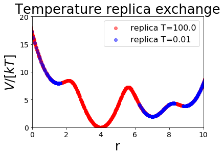
We now visualize which part of the potential energy surface our simulations sampled. For that reason, we color-code by the temperature of the replica. We start both replicas in the global minimum at \(r=4\). One replica is at the high temperature (T=4, red), one at the low temperature (T=0.1, blue). The replica at low temperature intensely samples this minimum, whereas the replica at high temperature is able to overcome the energy barriers surrounding the minimum. Therefore, only states from the high temperature replica are observed at the energy barriers.
After 200 steps the coordinates between our two simulations are exchanged. If the high temperature replica crossed the energy barrier before, the low temperature replica inherits these coordinates and starts in a different minimum. This minimum is then intensely sampled. Using multiple exchange trials, the low temperature replicate can sample all four minima without the need to cross the energy barriers in the low temperature replica.
[16]:
#plot
keys = sorted(list(replica_trajs.keys()), reverse=False)
positions = np.linspace(0,10)
fig, ax = plt.subplots(ncols=1)
# plot potential energy surface
ax.plot(positions, ensemble.replicas[0].potential.ene(positions), c="grey", alpha=0.7, zorder=-60)
colormap = { 0:'red', 1:'blue'}
for traj in keys:
T = round(ensemble.replicas[traj].temperature,2)
#min_e = np.min(replica_trajs[traj].total_potential_energy[eqil:])
ax.scatter(replica_trajs[traj].position, replica_trajs[traj].total_potential_energy, label="replica T="+str(T), c=colormap[traj], alpha=0.5)
ax.set_ylim([0,20])
ax.set_xlim([0,10])
ax.set_xlabel("r")
ax.set_ylabel("$V/[kT]$")
ax.legend()
ax.set_title("Temperature replica exchange")
fig.show()
C:\Users\benja\anaconda3\envs\EnsemblerDev\lib\site-packages\ipykernel_launcher.py:24: UserWarning: Matplotlib is currently using module://ipykernel.pylab.backend_inline, which is a non-GUI backend, so cannot show the figure.
Time-dependent bias
Time-dependent biasing methods update the bias during the simulation time. A frequently used time-dependent method is metadynamics/local elevation. There, a gaussian potential is added to the positions that were already visited during the simulation. Therefore, visiting these positions again, is energetically less favorable then in the previous visit (energetic penal).
Note, that in case of a Gaussian bias potential, the mean of the Gaussian is set to the current position of the particle and its width should be chosen small enough to avoid a big penal for neighboring states. Step by step the energetic minima are “flooded” and the particle can cross barriers more easily. In most applications the bias is only added every \(n^{th}\) step to iterate between free diffusion and biasing steps.
Metadynamics / Local elevation
We first define the original four-well potential. To apply metadynamics/local elevation we use the metadynamicsPotential function. In the initialization we have to define the height (\(amplitude\)) and width (\(sigma\)) of the gaussian bias function added. This bias potential is added every \(n\_trigger\) steps to the current position.
Adding more and more potentials every step leads to an energy function that demands more and more computation time every step. To avoid slowdown of the simulation the metadynamic bias is usually stored and calculated grid based. This allow a much faster simulation but comes at the cost of additional input parameter and small numerical errors in the bias force calculations. To initialize the grid, the user has to define the minimum x-position (\(bias\_grid\_min\)) and the maximum x-position (\(bias\_grid\_max\)) the grid should cover as well as the number of grid bins. Note, that no bias will be added to values below \(bias\_grid\_min\) or above \(bias\_grid\_max\).
In our example system we want to sample all four energy minima. Therefore, it is sufficient to set the grid between 0 and 10, which covers all four minima.
For the metadynamics/local elevation simulation we will reduce the simulation length by the factor of 10. This makes it easier to visually distinguish, and thus understand, the effect of metadynamics/local elevation.
[17]:
sim_steps = 200 # reduced simulation length
#Simulation Setup
origpot = fourWellPotential(Vmax=4, a=1.5, b=4.0, c=7.0, d=9.0, ah=2., bh=0., ch=0.5, dh=1.)
#Performe metadynamics
totpot = metadynamicsPotential(origpot, amplitude=.3, sigma=.21, n_trigger=10,
bias_grid_min=0, bias_grid_max=10, numbins=1000)
integrator = langevinIntegrator(dt=0.1, gamma=15)
system4=system(potential=totpot, sampler=integrator, start_position=4, temperature=1)
#simulate
cur_state = system4.simulate(sim_steps, withdraw_traj=True, init_system=False)
print("Trajectory length: ",len(system4.trajectory))
print()
print("last_state: ", cur_state)
print(len(system4.trajectory))
system4.trajectory.head()
Simulation: Simulation: 0%| | 0/200 [00:00<?, ?it/s]
initializing Langevin old Positions
Simulation: Simulation: 100%|██████████| 200/200 [00:02<00:00, 77.36it/s]
Trajectory length: 201
last_state: State(position=3.8428975757464716, temperature=1, total_system_energy=2.4687180714518107, total_potential_energy=2.4687180714518107, total_kinetic_energy=nan, dhdpos=0.8840124489125114, velocity=None)
201
[17]:
| position | temperature | total_system_energy | total_potential_energy | total_kinetic_energy | dhdpos | velocity | |
|---|---|---|---|---|---|---|---|
| 0 | 4.000000 | 1 | 0.003797 | -0.001344 | 0.005141 | 0.0034275749807509046 | 0.101399 |
| 1 | 3.999182 | 1 | 0.298541 | 0.298541 | NaN | -0.00342757 | NaN |
| 2 | 3.946611 | 1 | 0.303253 | 0.303253 | NaN | 0.0426495 | NaN |
| 3 | 3.974171 | 1 | 0.299241 | 0.299241 | NaN | 0.127614 | NaN |
| 4 | 4.072425 | 1 | 0.300863 | 0.300863 | NaN | 0.0388076 | NaN |
Metadynamic systems are visualized with the default simulation_analysis_plot function. simulation_analysis_plot will display the resulting potential after the last simulation step.
[18]:
#plot
simulation_analysis_plot(system4, title="position Langevin", limits_coordinate_space=list(range(0,10)))
[18]:
(<Figure size 1152x288 with 3 Axes>, None)
In the first panel of the visualization we can see how the system’s energy minimum around x=4 was flooded and the particle can cross neighboring energy barriers more easily. The longer one simulates, the flatter the whole energy surface become. Note however, that artifacts can arise once the system leaves the grid defined by \(bias\_grid\_min\) and \(bias\_grid\_max\). Therefore, these parameters have to be selected very carefully.
The Ensembler package also contains a build-in functionality to make short movies of the simulation using animation_trajectory. An example code is showing the beginning of the trajectory is given below.
[19]:
%matplotlib inline
import tempfile
from IPython.display import HTML
from ensembler.visualisation.animationSimulation import animation_trajectory, animation_EDS_trajectory
#plot simulation
ani, out_path = animation_trajectory(system4, limits_coordinate_space=list([0,8]), title="Awesome MetaDynamics",resolution_of_analytic_potential=1000)
##put it into jupyter:
os.chdir(tempfile.gettempdir())
x = ani.to_jshtml()
HTML(x)
[19]: