Conveyor Belt Thermodynamic Integration with Ensembler

In this notebook, we give examples how to run conveyor belt simulations with Ensembler.

Maintainers: [@SchroederB](https://https://github.com/SchroederB), [@linkerst](https://https://github.com/linkerst), [@dfhahn](https://https://github.com/dfhahn)

Loading Ensembler and necessary external packages

import os, sys
sys.path.append(os.getcwd()+"/..")

import numpy as np
import pandas as pd

import matplotlib.pyplot as plt
from matplotlib import cm
from matplotlib import colorbar
from mpl_toolkits.mplot3d import Axes3D

import ensembler.potentials.OneD as pot
import ensembler.system.perturbed_system as system
import ensembler.ensemble.replicas_dynamic_parameters as cvb
from ensembler.samplers import stochastic

Interactive Example

The following is an interactive example, which explains the concept of the conveyor belt algorithm

from ensembler.visualisation.interactive_plots import interactive_conveyor_belt

iwidget = interactive_conveyor_belt()
iwidget

Build a conveyor belt object

For building a conveyorBelt object, you first have to build a system, which will be used as a template for the replicas. The system itself needs to to be initialized with a potential and an integrator. For details, see the Tutorial Simulations.

sampler = stochastic.metropolisMonteCarloIntegrator()
potential = pot.linearCoupledPotentials(Va = pot.harmonicOscillatorPotential(k=1, x_shift=0.0),
    Vb = pot.harmonicOscillatorPotential(k=2, x_shift=2.0))
sys = system.perturbedSystem(potential=potential ,
                              sampler=sampler)

Additional the number of replicas n_replicas and the initial capital Lambda value needs to be specified. The latter can usually be set to 0. An additional (optional) argument is the build variable, which will be discussed later.

The output shows the current state of the conveyor belt as a table with the replica ID, the corresponding lambda value and the energy of the replica.

ensemble = cvb.conveyorBelt(capital_lambda=0.0,
                            n_replicas=4,
                            system=sys)
ensemble

i    lambda_i  E_i
-------------------------
    0      0.00    32.975
    1      0.50    32.975
    2      1.00    32.975
    3      0.50    32.975

Start a conveyor belt simulation

The conveyor belt is simulated by using its member function simulate with the number of steps as argument.

steps = 100
ensemble.simulate(steps)

The trajectories of the ensemble cvb_traj and the single systems sys_trajs can be retrieved by using its member function get_trajs.

(cvb_traj, systrajs) = ensemble.get_trajs()

The ensemble trajectory is a pandas.DataFrame object with the following columns: - Step: index of frame (starting from 1) - capital_lambda: the capital lambda of the frame - TotE: the current total energy of the ensemble - biasE: the current bias energy - doAccept: information whether the Monte Carlo step before the frame was accepted or not

cvb_traj.head()

	Step	capital_lambda	TotE	biasE	doAccept
0	0	0.000000	131.899937	0.0	True
1	0	5.539295	131.899937	0.0	True
2	1	5.249743	80.759163	0.0	True
3	2	5.748955	41.452370	0.0	True
4	3	6.149164	26.454378	0.0	True

The system trajectory object systrajs is a list of pandas.DataFrame objects (one per replica) with the following columns: - position: (spatial) position of particle - temperature: temperature - total_system_energy: the current total energy of the replica - total_potential_energy: the current potential energy of the replica - total_kinetic_energy: the current kinetic energy of the replica - dhdpos: the derivative of the hamiltonian with repect to the position (negative of the force) - velocity: velocity of the particle - lam: lambda value of the particle - dhdlam: Hamiltonian derivative with respect to lambda The kinetic energy and the velocity are NaN in the following, becauce this example uses the stochastic metropolisMonteCarloIntegrator, which does not calculate velocities.

systrajs[0].head()

	position	temperature	total_system_energy	total_potential_energy	total_kinetic_energy	dhdpos	velocity	lam	dhdlam
0	-3.478970704571898	298.0	11.726825	11.726825	NaN	1.7510607172656856	NaN	0.236788	23.967501
1	0.7551488977681826	298.0	0.701098	0.701098	NaN	4.234119602340081	NaN	0.328955	1.264529
2	0.44181625124460233	298.0	0.493877	0.493877	NaN	-0.3133326465235803	NaN	0.170051	2.330336
3	-0.4361344163389951	298.0	0.344227	0.344227	NaN	-0.8779506675835974	NaN	0.042660	5.839644
4	0.2002660837131477	298.0	0.395400	0.395400	NaN	0.6364005000521428	NaN	0.116604	3.218989

Visualizations of the trajectories

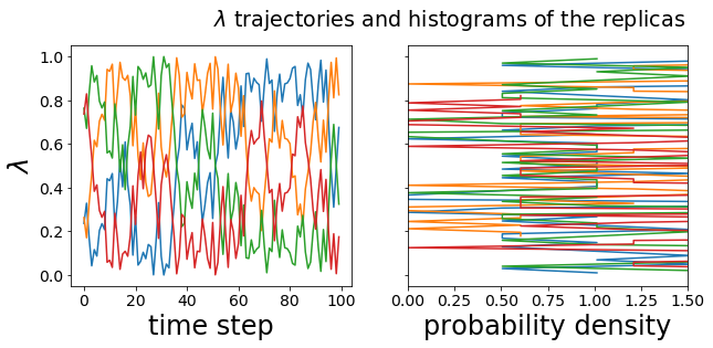
The following graph shows exemplarious the trajectories and histograms of the lambda variables of the single replicas. Other of the above mentioned variables can be plottet in the same way.

fig, ax = plt.subplots(1, 2, figsize=(10,4), sharey=True)
for i in systrajs:
    ax[0].plot(systrajs[i].index, systrajs[i].lam, label=f"{i}")
    h1=np.histogram(systrajs[i].lam, bins=50, density=1)
    ax[1].plot( h1[0], (h1[1][:-1]+h1[1][1:])/2)
ax[0].set_xlabel("time step")
ax[1].set_xlabel("probability density")
ax[0].set_ylabel("$\lambda$")
ax[1].set_xlim(0, 1.5)
out = plt.suptitle("$\lambda$ trajectories and histograms of the replicas", x=.6, y=1.0)

Simple analysis of the conveyor belt simulation

First, we simulate the conveyor belt even longer to get more statistics. Then, we sort the combined dhdlam trajectories from all replicas according to the associated lambda value. Then, we calculate the average per bin, which gives you the <dhdlam>(lam) estimate at point lam. In the following we use nbins=100, but you can adapt it according to your sampled data.

ensemble.simulate(900)
(cvb_traj, systrajs) = ensemble.get_trajs()

nbins=100
bins=np.zeros(nbins)
dhdlbins=np.zeros(nbins)
for i in systrajs:
    for j in range(systrajs[i].shape[0]):
        index=int(np.floor(systrajs[i].lam[j]*nbins))
        if index == nbins:
            index=nbins-1
        bins[index]+=1
        dhdlbins[index]+=systrajs[i].dhdlam[j]
# avoid division by zero by setting elements == 0 to 1
bins = np.where(bins, bins, 1)
dhdlbins/=bins

The plotted <dhdlam>(lam) curve is similar to the curves you get from TI simulations, but is usually base on more lambda points.

fig = plt.figure(figsize=(10,4))
plt.plot(np.linspace(0,1,nbins), dhdlbins)
plt.xlabel("$\lambda$")
plt.ylabel("$\partial H / \partial \lambda$")
out = plt.suptitle("$\partial H / \partial \lambda (\lambda)$ curve", x=.6, y=1.0)

The integral of this curve gives the free energy estimate. As you have many points along \(\lambda\), you can use the rectangular integration:

integral=np.sum(dhdlbins)*1.0/nbins
print(f'Delta G = {integral:.2f} kJ/mol')

This value agrees well to the analytical value, which is calculated below.

#analytical
u=1.66053886e-27
NA=6.0221415e23
hbar=1.054571800e-34*1e12*1e-3*NA  #kJ/mol*ps
R=0.00831446 #kJ/mol/K
mu=0.5  #u
T=298.0  #K
fc1=1  #kJ/nm^2/mol
fc2=2.0 #kJ/nm^2/mol
omega1=np.sqrt(fc1/mu)
omega2=np.sqrt(fc2/mu)
alpha1=hbar*np.sqrt(fc1/mu)/(R*T)
alpha2=hbar*np.sqrt(fc2/mu)/(R*T)
Z1=np.exp(-alpha1/2.0)/(1-np.exp(-alpha1))
Z2=np.exp(-alpha2/2.0)/(1-np.exp(-alpha2))
DF=-R*T*np.log(Z2/Z1)
print(f'Analytical value = {DF:.2f} kJ/mol')