Potentials¶

In this Notebook you can find the different Potentials, that are already implemented and can be used for your projects. Play around with the parameters to get familiar with the Potentials

Here you also can find classical Potentials like the harmonic Oscillator or the Lennard Jones Potential.

[1]:

#if the package was not installed:
import os, sys
path = "../"
sys.path.append(path)

#Imports
##general
import numpy as np
from matplotlib import pyplot as plt

##Ensembler
from ensembler.potentials import OneD as potentials1D
from ensembler.potentials import TwoD as potentials2D

import ensembler.visualisation.plotPotentials as vis

###Plotting:

#params
test_timing_with_points =1000

Classics¶

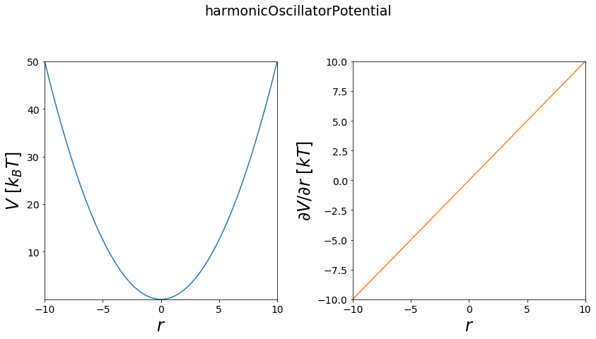
Harmonic Oscillator¶

The Harmonic Oscillator is one of the most used modelling potentials1D. Its based on hooke’s law and can be used to describe obviously springs, but also covalent bonds of two atoms and many more physical relations.

Functional:

\(V = \frac{1}{2}*k*(r - r_0)^2+V_{offset}\)

with: * \(k\) force constant * \(r_0\) optimal position (optimal covalent bond length) * \(r\) current position (current bond length) * \(V_{offset}\) minimal potential energy offset

first partial derivative by r

\(\frac{\partial V}{\partial r} = k*(r - r_0)\)

1D¶

[3]:

# 1D
positions = np.linspace(-10,10, test_timing_with_points)

V = potentials1D.harmonicOscillatorPotential()
#print(V)

print("calculate "+str(len(positions))+" positions: ")
%time V.ene(positions)

print("\nVisualization")
fig, axes = vis.plot_potential(V, positions=positions)

calculate 1000 positions:
Wall time: 0 ns

Visualization

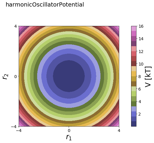
../_images/Tutorials_Tutorial_Potentials_4_1.png

2D¶

[4]:

# 2D
positions = np.linspace(-4, 4, test_timing_with_points)
x_positions, y_positions = np.meshgrid(positions,positions)
positions2D = np.array([x_positions.flatten(), y_positions.flatten()]).T

V = potentials2D.harmonicOscillatorPotential()
#print(V)

print("calculate "+str(len(positions))+" positions: ")
%time V.ene(positions2D)


print("\nVisualization")
positions = np.linspace(-4, 4, test_timing_with_points)
x_positions, y_positions = np.meshgrid(positions,positions)
positions2D = np.array([x_positions.flatten(), y_positions.flatten()]).T

fig, axes = vis.plot_potential(V, positions2D)

calculate 1000 positions:
Wall time: 64.7 ms

Visualization

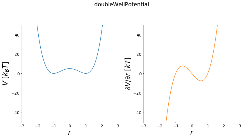
../_images/Tutorials_Tutorial_Potentials_6_1.png

Double Well Potential¶

The double well potential can be used to simulate a system with two states continously. For example in chemistry this can be used as a toy model for the transition of protonation states of a single protonatable molecule. (see Donnini 2016)

Functional:

\(V = \frac{V_{max}}{b^4}*((-\frac{a}{2} + r)^2-b^2)^2\)

first order derivative

\(\frac{\partial V}{\partial r} = \frac{V_max}{b^4}*(-2a + 4r)*((-a/2 + r)^2-b^2)\)

[5]:

positions = np.linspace(-3, 3, test_timing_with_points)

V = potentials1D.doubleWellPotential(a=0, b=1, Vmax=5)
#print(V)

print("calculate "+str(len(positions))+" positions: ")
%time V.ene(positions)

print("\nVisualization")
fig, axes = vis.plot_potential(V, positions=positions, y_range=[-50,50])

pass

calculate 1000 positions:
Wall time: 1.36 ms

Visualization

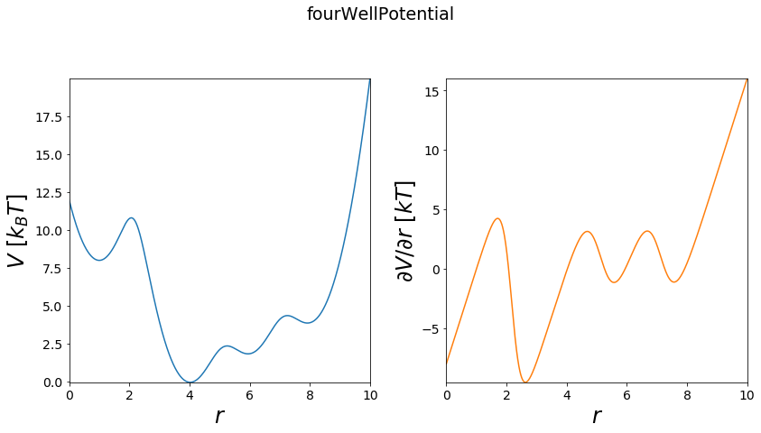
../_images/Tutorials_Tutorial_Potentials_8_1.png

Four Well Potential¶

The four well can be understood as a expansion of the double well potential, and can be used for simulations with four states.

[6]:

#phase space
positions = np.linspace(0, 10, test_timing_with_points)

#build potential
V = potentials1D.fourWellPotential(a=1,b=4, c=6, d=8)

print("calculate "+str(len(positions))+" positions: ")
%time V.ene(positions)

print("\nVisualization") #visualize
fig, axes = vis.plot_potential(V, positions=positions)
#fig.savefig("four_well.png")

pass

calculate 1000 positions:
Wall time: 950 µs

Visualization

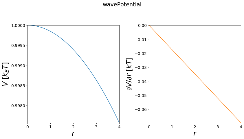
../_images/Tutorials_Tutorial_Potentials_10_1.png

Wave Potential¶

Wave potentials are typically used in chemical modelling for torsion angles.

Functional:

\(A*cos(m*(r + w)) + V_{off}\)

first derivative:

\(\frac{\partial V}{\partial r} = -A*m*sin(m*(r + w))\)

[7]:

#1D
positions = np.linspace(0, 4, test_timing_with_points)

V = potentials1D.wavePotential()
#print(V)

print("calculate "+str(len(positions))+" positions: ")
%time V.ene(positions)

print("\nVisualization")
fig, axes = vis.plot_potential(V, positions=positions)

calculate 1000 positions:
Wall time: 992 µs

Visualization

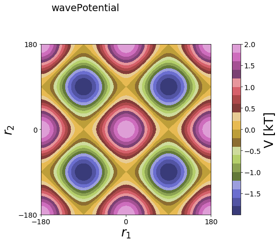
../_images/Tutorials_Tutorial_Potentials_12_1.png

2D¶

[8]:

positions = np.linspace(-180, 180, test_timing_with_points)
x_positions, y_positions = np.meshgrid(positions,positions)
positions2D = np.array([x_positions.flatten(), y_positions.flatten()]).T

V = potentials2D.wavePotential(multiplicity=[2,2], radians=False)
#print(V)

print("calculate "+str(len(positions))+" positions: ")
%time V.ene(positions2D)


print("\nVisualization")
fig, axes = vis.plot_potential(V, positions2D)

calculate 1000 positions:
Wall time: 226 ms

Visualization

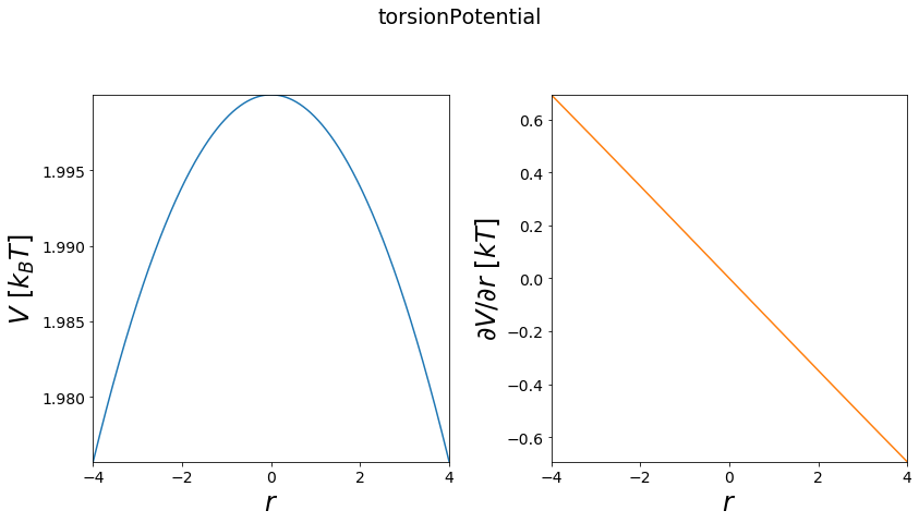
../_images/Tutorials_Tutorial_Potentials_14_1.png

Torsion Potential¶

The Torsion potential is an overlay of multiple wave potentials and can be used to build more complex torsion potentials, hence the name.

[9]:

positions = np.linspace(-4, 4, test_timing_with_points)

w1 = potentials1D.wavePotential(multiplicity=3)
w2 = potentials1D.wavePotential()
waves = [w1, w2]

V = potentials1D.torsionPotential(wavePotentials=waves)
#print(V)

print("calculate "+str(len(positions))+" positions: ")
%time V.ene(positions)

print("\nVisualization")
fig, axes = vis.plot_potential(V, positions=positions)

calculate 1000 positions:
Wall time: 2.09 ms

Visualization

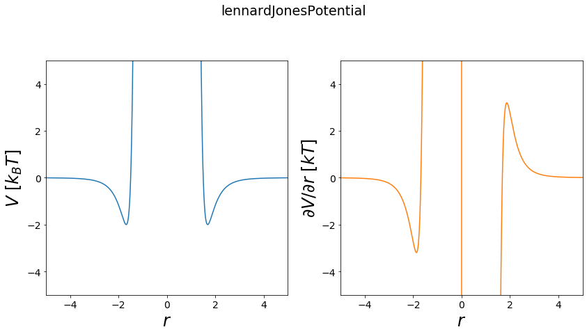
../_images/Tutorials_Tutorial_Potentials_16_1.png

Lennard Jones Potential¶

The lennard jones potential is used usally to describe the Van der Waals terms between multiple atoms. On long distances between two atoms the potential converges to zero, so the atoms don’t “see” each other anymore. On very short distances between two atoms the potential goes to infinity, representing a huge energy barrier. The minimum of the potential represents the optimal distance of the two atoms.

Functional:

\(V = 4e*(\frac{s^{12}}{(r - r_0)^12} - \frac{s^6}{(r - r_0)^6}) + V_{off}\)

first derivative:

\(\frac{\partial V}{\partial r} = 4e*(-12*\frac{s^{12}}{(r - r_0)^13} + 6*\frac{s^6}{(r - r_0)^7})\)

[10]:

positions = np.linspace(-5, 5, test_timing_with_points)

V = potentials1D.lennardJonesPotential()
#print(V)

print("calculate "+str(len(positions))+" positions: ")
%time V.ene(positions)

print("\nVisualization")
fig, _ = vis.plot_potential(V, positions=positions, y_range=[-5,5])
pass

calculate 1000 positions:
Wall time: 1.15 ms

Visualization

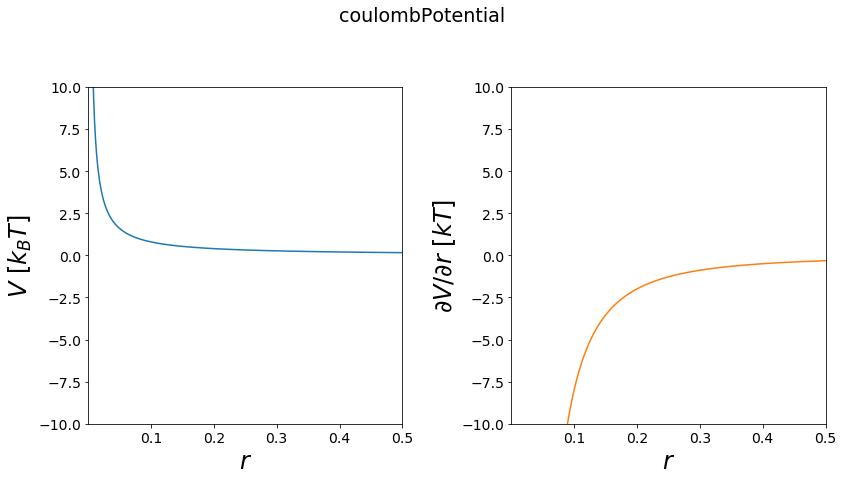
../_images/Tutorials_Tutorial_Potentials_18_1.png

Culomb Potential¶

Culomb potentials are used in chemical modelling for the representation of charged interatctions between two non-bonded atoms.

Functional:

\(V = \frac{q_1q_2}{(4 \pi \epsilon r)}\)

first derivative:

\(\frac{\partial V}{\partial r} = \frac{-q_1q_2}{(4\pi \epsilon r^2)}\)

[11]:

positions = np.linspace(0.00001, 0.5, test_timing_with_points)

V = potentials1D.coulombPotential()
#print(V)

print("calculate "+str(len(positions))+" positions: ")
%time V.ene(positions)

print("\nVisualization")
fig, axes = vis.plot_potential(V, positions=positions, y_range=[-10,10])

calculate 1000 positions:
Wall time: 0 ns

Visualization

../_images/Tutorials_Tutorial_Potentials_20_1.png

Perturbed/MultiState Potentials¶

For free energy calculations the potentials of two states can be coupled to each other. Two general approaches of such potential coupling schemes are shown here. If you want to learn more about their usage and free energy calculations, checkout the Free Energy Calculation Jupyter-Notebook.

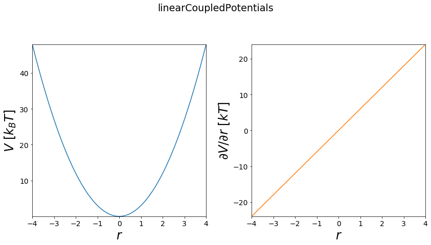
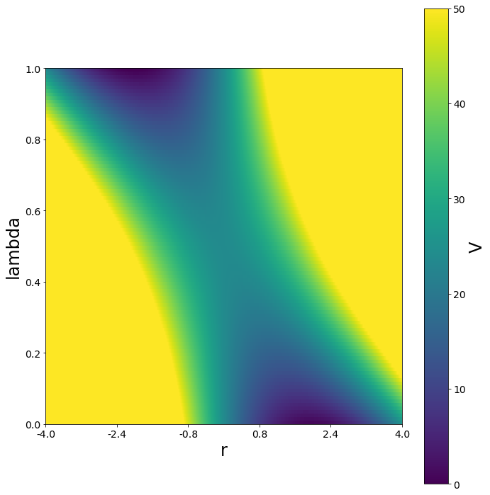
linear coupled¶

The linear coupling uses a \(\lambda\)-variable to couple the two potentials \(V_a\) and \(V_b\) in a linear combination. Here a \(\lambda = 1\) stands for a pure \(V_a\) and a \(\lambda = 0\) for a pure \(V_b\). The ideal mixture of states is reached with \(\lambda = 0.5\) and all other \(\lambda\)s between \([0,1]\) are representing intermediate states between \(V_a\) and \(V_b\).

Functional:

\(V(r, \lambda) = \lambda V_a(r) + (1-\lambda) V_b(r)\)

first order derivatives:

\(\frac{\partial V}{\partial \lambda} = V_a - V_b\)

\(\frac{\partial V}{\partial r} = \lambda \frac{\partial V_a(r)}{\partial r} - (1-\lambda) \frac{\partial V_b(r)}{\partial r}\)

[12]:

positions = np.linspace(-4, 4, test_timing_with_points)

w1 = potentials1D.harmonicOscillatorPotential()
w2 = potentials1D.harmonicOscillatorPotential(k=11)

V = potentials1D.linearCoupledPotentials(Va=w1, Vb=w2)
#print(V)

print("calculate "+str(len(positions))+" positions: ")
%time V.ene(positions)

print("\nVisualization")
fig, axes = vis.plot_potential(V, positions=positions)

calculate 1000 positions:
Wall time: 0 ns

Visualization

../_images/Tutorials_Tutorial_Potentials_23_1.png

[13]:

positions = np.linspace(-4, 4, test_timing_with_points)

w1 = potentials1D.harmonicOscillatorPotential(k=10, x_shift=-2)
w2 = potentials1D.harmonicOscillatorPotential(k=10, x_shift=2)


w1 = potentials1D.harmonicOscillatorPotential(k=12, x_shift=-2)
w2 = potentials1D.harmonicOscillatorPotential(k=12, x_shift=2)
V = potentials1D.linearCoupledPotentials(Va=w1, Vb=w2)

lambda_ene = []
for lam in np.arange(0, 1, 0.01):
    V.set_lambda(lam)
    lambda_ene.append(V.ene(positions))

print("\nVisualization")
fig, ax = plt.subplots(ncols=1, figsize=[10,10])
mapping = ax.imshow(lambda_ene, extent=[0,100, 0,100], vmin=0, vmax=50)
opt_labels = np.array(ax.get_yticks())/100
ax.set_yticklabels(opt_labels)
opt_labels = np.round(((np.array(ax.get_yticks())/100)*8)-4,2)
ax.set_xticklabels(opt_labels)

ax.set_ylabel("lambda")
ax.set_xlabel("r")
cm = plt.colorbar(mapping)
cm.set_label("V")
fig.tight_layout()


Visualization

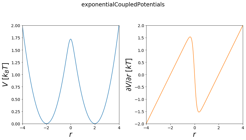
../_images/Tutorials_Tutorial_Potentials_24_1.png

exponential Copuled - Enveloping Potential¶

This way of coupling is used in enveloping distribution sampling (EDS). The coupling scheme is generating an artificial reference state, via summing the end potentials in a log-sum-exp operation. The reference state contains two parameters the smoothing parameter \(s\) and the energy offset vector \(E^R\).

Functional:

\(V(r) = -\frac{1}{k_b T s} ln(e^{- k_b T s (V_i-E^{off}_i)}+e^{-k_b T s (V_j-E^{off}_j)})\)

[14]:

positions = np.linspace(-4, 4, test_timing_with_points*10000)

w1 = potentials1D.harmonicOscillatorPotential(x_shift=-2)
w2 = potentials1D.harmonicOscillatorPotential(x_shift=2)

#print(w1, w2)
V = potentials1D.exponentialCoupledPotentials(Va=w1, Vb=w2, s=1, eoffA=0, eoffB=0)
#print(V)

print("calculate "+str(len(positions))+" positions: ")
%time V.ene(positions)

print("\nVisualization")
fig, axes = vis.plot_potential(V, positions=positions)
plt.show()
plt.close()
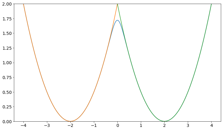
plt.plot(positions, V.ene(positions))
plt.plot(positions, w1.ene(positions))
plt.plot(positions, w2.ene(positions))
plt.ylim([0,2])

calculate 10000000 positions:
Wall time: 2.15 s

Visualization

../_images/Tutorials_Tutorial_Potentials_26_1.png

[14]:

(0, 2)

../_images/Tutorials_Tutorial_Potentials_26_3.png

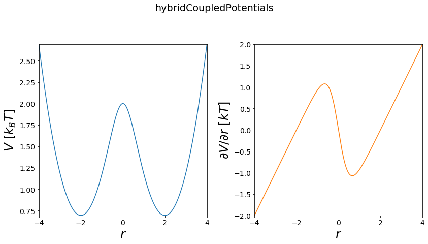
linear & exponential hybrid Copuled - \(\lambda\) EDS¶

This is a generalization, combining both previously introduced coupling schemes into one.

Functional:

\(V(r) = -\frac{1}{k_b T s} ln(\lambda e^{- k_b T s (V_i-E^{off}_i)}+(1-\lambda)e^{-k_b T s (V_j-E^{off}_j)})\)

[15]:

positions = np.linspace(-4, 4, test_timing_with_points)

w1 = potentials1D.harmonicOscillatorPotential(x_shift=-2)
w2 = potentials1D.harmonicOscillatorPotential(x_shift=2)

V = potentials1D.hybridCoupledPotentials(Va=w1, Vb=w2, lam=0.5)
#print(V)

print("calculate "+str(len(positions))+" positions: ")
%time V.ene(positions)

print("\nVisualization")
fig, axes = vis.plot_potential(V, positions=positions)
plt.show()
plt.close()
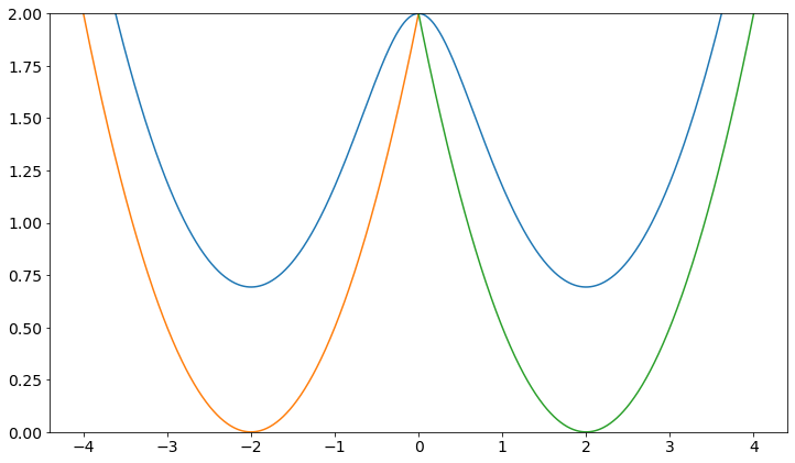
plt.plot(positions, V.ene(positions))
plt.plot(positions, w1.ene(positions))
plt.plot(positions, w2.ene(positions))

plt.ylim([0,2])


#perturbed potentilas

calculate 1000 positions:
Wall time: 0 ns

Visualization

../_images/Tutorials_Tutorial_Potentials_28_1.png

[15]:

(0, 2)

../_images/Tutorials_Tutorial_Potentials_28_3.png

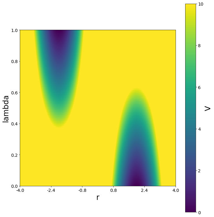
Next we will show, how the system changes with \(\lambda\).

[16]:

positions = np.linspace(-4, 4, test_timing_with_points)

w1 = potentials1D.harmonicOscillatorPotential(k=12, x_shift=-2)
w2 = potentials1D.harmonicOscillatorPotential(k=12, x_shift=2)
V = potentials1D.hybridCoupledPotentials(Va=w1, Vb=w2, s=0.1)

lambda_ene = []
for lam in np.arange(0, 1.01, 0.01):
    V.set_lambda(lam)
    lambda_ene.append(V.ene(positions))

print("\nVisualization")
fig, ax = plt.subplots(ncols=1, figsize=[10,10])
mapping = ax.imshow(lambda_ene, extent=[0,100, 0,100], vmin=0, vmax=10)
opt_labels = np.array(ax.get_yticks())/100
ax.set_yticklabels(opt_labels)
opt_labels = np.round(((np.array(ax.get_yticks())/100)*8)-4,2)
ax.set_xticklabels(opt_labels)

ax.set_ylabel("lambda")
ax.set_xlabel("r")
cm = plt.colorbar(mapping)
cm.set_label("V")
fig.tight_layout()


Visualization

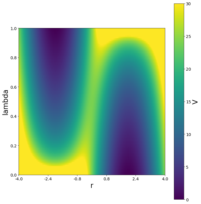
../_images/Tutorials_Tutorial_Potentials_30_1.png

To smoothen the transition and lowering the barrier between the states, the \(\lambda\) and the s parameter can be changed simultaneosly.

[17]:

positions = np.linspace(-4, 4, test_timing_with_points)

w1 = potentials1D.harmonicOscillatorPotential(k=12, x_shift=-2)
w2 = potentials1D.harmonicOscillatorPotential(k=12, x_shift=2)
V = potentials1D.hybridCoupledPotentials(Va=w1, Vb=w2, s=0.1)


points=50
lambda_ene = []
for lam, s in zip(np.linspace(0, 0.5, points), np.logspace(0, -3,  points)):
    V.set_lambda(lam)
    V.s=s
    lambda_ene.append(V.ene(positions))
for lam, s in zip(np.linspace(0.51, 1,  points), np.logspace(-3, 0,  points)):
    V.set_lambda(lam)
    V.s=s
    lambda_ene.append(V.ene(positions))

print("\nVisualization")
fig, ax = plt.subplots(ncols=1, figsize=[10,10])
mapping = ax.imshow(lambda_ene, extent=[0,100, 0,100], vmin=0, vmax=30)
opt_labels = np.array(ax.get_yticks())/100
ax.set_yticklabels(opt_labels)
opt_labels = np.round(((np.array(ax.get_yticks())/100)*8)-4,2)
ax.set_xticklabels(opt_labels)

ax.set_ylabel("lambda")
ax.set_xlabel("r")
cm = plt.colorbar(mapping)
cm.set_label("V")
fig.tight_layout()


Visualization

../_images/Tutorials_Tutorial_Potentials_32_1.png

Special Potentials¶

The Gerhard Koenig speciality corner. Here we have some special potential for very special usecases.

dummy Potential¶

This potential returns always the same value independt on its position.

[18]:

positions = np.linspace(1,100, test_timing_with_points)

V = potentials1D.dummyPotential()

print("calculate "+str(len(positions))+" positions: ")
%time V.ene(positions)

print("\nVisualization")
fig, axes = vis.plot_potential(V, positions=positions)

calculate 1000 positions:
Wall time: 0 ns

Visualization

..\ensembler\visualisation\plotPotentials.py:84: UserWarning: Attempting to set identical bottom == top == 0 results in singular transformations; automatically expanding.
  ax.set_ylim(min(y_range), max(y_range)) if (y_range != None) else ax.set_ylim(min(energies), max(energies))
..\ensembler\visualisation\plotPotentials.py:111: UserWarning: Attempting to set identical bottom == top == 0.0 results in singular transformations; automatically expanding.
  ax.set_ylim(min(y_range), max(y_range)) if (y_range != None) else ax.set_ylim(min(energies), max(energies))

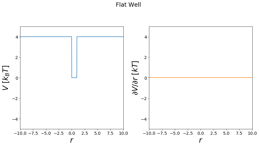
../_images/Tutorials_Tutorial_Potentials_35_2.png

Flatwell Potential¶

A potential return dependent on a position a value in a binary fashion

[19]:

positions = np.linspace(-10,10, test_timing_with_points)

V = potentials1D.flatwellPotential(y_min=0)

print("calculate "+str(len(positions))+" positions: ")
%time V.ene(positions)

print("\nVisualization")
fig, _ = vis.plot_potential(V, positions=positions, y_range=[-5,5])

calculate 1000 positions:
Wall time: 2.55 ms

Visualization

../_images/Tutorials_Tutorial_Potentials_37_1.png